What is `process_data()`?

process_data() converts raw population counts into a sampled data frame (one row per icon) ready for geom_pop().

It handles:

Calculating group proportions from raw counts
Proportionally allocating a fixed sample size across groups
Supporting hierarchical grouping via high_group_var

library(ggpop)
library(ggplot2)
library(dplyr)

Basic Usage

Required: data, group_var, sum_var. sample_size sets icon count (max 1,000).

df_sex <- data.frame(
  sex = c("male", "female"),
  n   = c(63459580, 67401427)
)

df_sex_proc <- process_data(
  data        = df_sex,
  group_var   = sex,
  sum_var     = n,
  sample_size = 100
)

head(df_sex_proc)

    type        n      prop
1   male 63459580 0.4849388
2   male 63459580 0.4849388
3   male 63459580 0.4849388
4 female 67401427 0.5150612
5 female 67401427 0.5150612
6   male 63459580 0.4849388

The output contains:

type: group label (from group_var)
n: total count for that group
prop: proportion of the total
One row per sampled icon

Understanding Proportions

With sample_size = 100, a group with 48% of the population gets ~48 icons.

df_sex_proc %>%
  group_by(type) %>%
  summarise(
    icons      = n(),
    proportion = round(mean(prop) * 100, 1)
  )

# A tibble: 2 × 3
  type   icons proportion
  <chr>  <int>      <dbl>
1 female    54       51.5
2 male      46       48.5

Multiple Groups

Works with any number of groups — not just two.

df_regions <- data.frame(
  region = c("North", "South", "East", "West"),
  n      = c(12000, 8000, 15000, 5000)
)

df_regions_processed <- process_data(
  data        = df_regions,
  group_var   = region,
  sum_var     = n,
  sample_size = 100
)

df_regions_processed %>%
  group_by(type) %>%
  summarise(icons = n())

# A tibble: 4 × 2
  type  icons
  <chr> <int>
1 East     31
2 North    33
3 South    20
4 West     16

Hierarchical Grouping with `high_group_var`

Use high_group_var to nest groups under a parent category for faceted plots.

df_health <- data.frame(
  region    = c("North", "South", "East", "West",
                "North", "South", "East", "West"),
  status    = c(rep("Healthy", 4), rep("At Risk", 4)),
  n         = c(8000, 6000, 9000, 4000,
                4000, 2000, 6000, 1000)
)

df_health_processed <- process_data(
  data           = df_health,
  group_var      = status,
  sum_var        = n,
  high_group_var = "region",
  sample_size    = 100
)

df_health_processed %>%
  group_by(group, type) %>%
  summarise(icons = n(), .groups = "drop")

# A tibble: 8 × 3
  group type    icons
  <chr> <chr>   <int>
1 East  At Risk    39
2 East  Healthy    61
3 North At Risk    32
4 North Healthy    68
5 South At Risk    24
6 South Healthy    76
7 West  At Risk    14
8 West  Healthy    86

Skipping `process_data()`

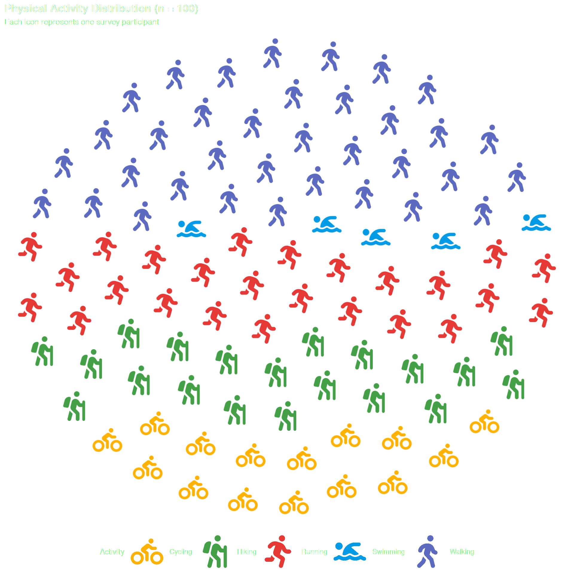
Optional — pass data directly to geom_pop() if it already has one row per icon (max 1,000 rows per plot or facet).

df_direct <- data.frame(
  activity = c(
    rep("Walking",  35),
    rep("Running",  25),
    rep("Hiking",   20),
    rep("Cycling",  15),
    rep("Swimming",  5)
  ),
  icon = c(
    rep("person-walking",  35),
    rep("person-running",  25),
    rep("person-hiking",   20),
    rep("person-biking",   15),
    rep("person-swimming",  5)
  )
)

# Pass directly — no process_data() needed
ggplot() +
  geom_pop(
    data = df_direct,
    aes(icon = icon, color = activity),
    size = 2, dpi = 100, legend_icons = TRUE, arrange = TRUE
  ) +
  scale_color_manual(values = c(
    "Walking"  = "#5C6BC0",
    "Running"  = "#E53935",
    "Hiking"   = "#43A047",
    "Cycling"  = "#FFB300",
    "Swimming" = "#039BE5"
  )) +
  theme_pop() +
  theme(plot.title = element_text(color = "white"),
        plot.subtitle = element_text(color = "white"),
        legend.text = element_text(color = "white"),
        legend.title = element_text(color = "white"),
        legend.position = "bottom") +
  scale_legend_icon(size = 8) +
  labs(
    title    = "Physical Activity Distribution (n = 100)",
    subtitle = "Each icon represents one survey participant",
    color    = "Activity"
  )

Summary

Parameter	Description
`data`	Input data frame with group counts
`group_var`	Column to group by (unquoted)
`sum_var`	Column with population counts
`sample_size`	Number of icons to generate (max 1,000)
`high_group_var`	Optional parent grouping for faceting

Preparing Data with process_data()

What is process_data()?